Evaluation of Semi-automatic Segmentation Methods for Persistent Ground Glass Nodules on Thin-Section CT Scans

Article information

Healthc Inform Res. 2016;22(4):305-315

Publication date (electronic) : 2016 October 31

doi : https://doi.org/10.4258/hir.2016.22.4.305

Young Jae Kim, MS ¹^,², Seung Hyun Lee, PhD ², Chang Min Park, MD ³, Kwang Gi Kim, PhD ¹

¹Biomedical Engineering Branch, Division of Precision Medicine and Cancer Informatics, Research Institute, National Cancer Center, Goyang, Korea.

²Department of Plasma Bio Display, Kwangwoon University, Seoul, Korea.

³Department of Radiology, Seoul National University Hospital, Seoul, Korea.

Corresponding Author: Kwang Gi Kim, PhD. Biomedical Engineering Branch, Division of Precision Medicine and Cancer Informatics, Research Institute, National Cancer Center, 323 Ilsan-ro, Ilsandong-gu, Goyang 10408, Korea. Tel: +82-31-920-2241, kimkg@ncc.re.kr

Received 2016 September 17; Revised 2016 September 27; Accepted 2016 September 29.

Abstract

Objectives

This work was a comparative study that aimed to find a proper method for accurately segmenting persistent ground glass nodules (GGN) in thin-section computed tomography (CT) images after detecting them.

Methods

To do this, we first applied five types of semi-automatic segmentation methods (i.e., level-set-based active contour model, localized region-based active contour model, seeded region growing, K-means clustering, and fuzzy C-means clustering) to preprocessed GGN images, respectively. Then, to measure the similarities, we calculated the Dice coefficient of the segmented area using each semiautomatic method with the result of the manually segmented area by two radiologists.

Results

Comparison experiments were performed using 40 persistent GGNs. In our experiment, the mean Dice coefficient for each semiautomatic segmentation tool with manually segmented area was 0.808 for the level-set-based active contour model, 0.8001 for the localized region-based active contour model, 0.629 for seeded region growing, 0.7953 for K-means clustering, and 0.7999 for fuzzy C-means clustering, respectively.

Conclusions

The level-set-based active contour model algorithm showed the best performance, which was most similar to the result of manual segmentation by two radiologists. From the differentiation between the normal parenchyma and the nodule, it was also the most efficient. Effective segmentation methods will be essential for the development of computer-aided diagnosis systems for more accurate early diagnosis and prognosis of lung cancer in thin-section CT images.

Keywords: Lung; Computer-Assisted Image Processing; Solitary Pulmonary Nodule; Computer-Assisted Diagnosis; X-Ray Computed Tomography Scanners

I. Introduction

Lung cancer is the leading cause of death due to malignancy in most countries, with more than 1.3 million deaths estimated worldwide and 160,000 deaths estimated in the United States annually for both men and women [1]. Moreover, the death toll due to lung cancer is higher than the total number of deaths due to prostate, breast, and colorectal cancer, which have higher incidences than lung cancer. The high rate of death for lung cancer patients is due to the late diagnosis of more than 75% of patients with advanced lung cancer, in which curative treatment is impossible. Therefore, the development of a cancer marker capable of detecting cancer in its early stage is urgently required to improve the treatment and prognosis of lung cancer patients [2].

A ground-glass nodule (GGN) is defined as a nodule that has an internal density without obscuring the underlying pulmonary vessels within the nodule. The presence of GGNs in computed tomography (CT) scans often leads to more diagnostic evaluations, including lung biopsies [3]. Although GGNs are non-specific findings in general, persistent GGNs on CT scans raise the possibility of a typical adenomatous hyperplasia (AAH), bronchioloalveolar cell carcinoma (BAC), adenocarcinoma, and focal interstitial fibrosis with chronic inflammation (FIF). AAH is defined as a lesion with a well-defined boundary produced by the proliferation of monotonous, minimally atypical columnar epithelial cells along alveoli and respiratory bronchioles. BAC is defined as adenocarcinoma with a pure bronchioloalveolar growth pattern and no evidence of stromal, vascular, or pleural invasion [4]. AAH and localized BAC are usually manifested by a pure GGN, whereas more advanced adenocarcinoma may include a larger solid component within the region of the GGN [5].

The areas of GGNs or disappearing areas on mediastinal window images in lung adenocarcinomas in thin-section CT scans correspond to the areas of the BAC component on histopathological examination [6].

The possibility of lung cancer needs to be considered if GGN persists over follow-ups. Pure GGNs that are larger than 10 mm in size should be assumed as BAC or invasive adenocarcinoma if they persist for at least 3 months. Part-solid GGNs having an internal solid component have been reported to have a much higher cancer probability, and they are presumed to be malignant, which justifies surgical resection [7].

In clinical practice, the detection and characterization of GGNs is solely based on subjective assessment by experts. However, the detection of faint abnormal regions, such as GGNs, can be very difficult and time-consuming since GGNs are usually small and show contrast with the surrounding lung parenchyma.

To overcome these limitations, various efforts have been made in the development of computer-aided diagnosis (CAD) systems for detecting GGN regions in CT images [8 9]. Currently, the typical performance of CAD schemes in thick-section CT is a sensitivity of approximately 80%–90% with 1–2 false positives per section, which translates into tens of false positives per CT scan [10]. In addition to GGN detection, the recognition of lesion growth in a follow-up of GGN is also an important factor in determining time for the accurate diagnosis of lung cancers manifesting as GGNs and their corresponding prompt treatment.

Since the measurement of lesions is based on visual inspection, this can lead to a considerable amount of error; thus, computerized quantification, which is more reproducible, is expected to be a promising measurement of lesion growth over time.

Most research related to CAD systems has been essentially based on various image processing techniques, such as geometrical modeling, clustering, spatial filtering, etc. [11 12].

For example, Zhou et al. [13] proposed a new algorithm that detects GGN regions using the boosted K-nearest neighbor (K-NN) technique and segments them automatically using a three-dimensional (3D) texture likelihood map. As a test result from 200 volume samples, their method achieved an average error rate of 3.7% from the boosted K-NN classifier. All regions with one false positive region were detected accurately from a volume data with 10 GGN regions. In this study, the assessment of detection performance was conducted, but there was no quantitative evaluation of accuracy regarding image segmentation. Kim et al. [14] also proposed a new algorithm for detecting and segmenting GGNs, which combined statistical features and artificial neural networks (ANNs). A test result from 31 CT cases showed a sensitivity of about 82% and a scan per FP rate of 1.07, respectively.

As a similar approach, Bastawrous et al. [15] extracted features using the Gabor filter, followed by classifications using ANNs and a template matching algorithm. In the case of ANN, they achieved a sensitivity of 84% and a FP rate of 0.25, while the case of template matching showed a sensitivity of 92% and an FP rate of 0.76, respectively. However, their approach needs an extra step of region-of-interest (ROI) setting for each slice in advance, and preprocessing is very time consuming.

Ikeda et al. performed research on the analysis of CT numbers to discriminant AAH, BAC, and adenocarcinoma on CT scans, and to determine optimal cutoff CT number values [16]. In this research, the discrimination between AAH and BAC showed high values, with a sensitivity of 0.90 and a specificity of 0.81, respectively. Although they also reported that CT numbers can be used as effective parameters in the case regarding the discrimination between BAC and adenocarcinomas, the discrimination between BAC and adenocarcinoma achieved relatively low values, with a sensitivity of 0.75 and a specificity of 0.81, respectively. In addition, their method is very time consuming for the acquisition of related information on 3D volume data.

Most of these CAD schemes exclude the segmentation of GGNs and focus on the detection of nodules only. However, in the computer-based detection of lung nodules, such as GGNs, to obtain high accuracy, it is important to use effective image segmentation methods during the major steps of the detection scheme; if clinicians try to perform a postoperative follow-up study for predicting the prognosis of lung cancer, the accurate segmentation of lesions should be carried out prior to the extraction and analysis of CAD features.

Therefore, in this study, we evaluated their suitability in CAD systems through a comparative study of GGN segmentation results for CT scans obtained by manual segmentation and semi-automatic segmentation methods (i.e. level-set-based active contour model, localized region-based active contour model, seeded region growing, K-means, and fuzzy C-means clustering).

The remained of this paper is organized as follows. Section II describes the research along with the details of how the images used in the experiment and methods were obtained. Section III presents the study results from the application of methods to the actual clinical data. Finally, Section IV evaluates the results of the study and suggests a direction for further studies.

II. Methods

Figure 1 describes the detailed three-step approach adopted in this research, related to the segmentation and evaluation of its results.

Figure 1

Overall procedure of the study.

First, we performed image acquisition and preprocessing steps. Then, we segmented the clinical test image data with five types of semi-automatic segmentation methods. Finally, for quantitative evaluation, we calculated indices in diverse forms from statistical analysis.

1. CT Scanning

Axial lung CT scans were obtained from two CT scanners in the Department of Radiology, Seoul National University Hospital: Sensation-16, Somatom Plus 4 (Siemens Medical Systems, Erlangen, Germany), LightSpeed Ultra, and HiSpeed Advantage (GE Medical Systems, Milwaukee, WI, USA). More detailed scanning parameters are summarized as follows. The tube voltage was 120 kVp, and the X-ray tube currents were in the range of 100–200 mA. Slice thicknesses were 1.0–1.25 mm. The image resolution and size were 1.467 pixels per mm and 0.68 × 0.6 mm, respectively. The size of each scan was 512 × 512 with 12 bits per pixel. We obtained a total of four data sets, which consisted of about 15–40 slices, and we used a total 40 images containing nodules, which were randomly selected for testing the segmentation methods. Clinical and radiologic diagnoses were made by two experienced radiologists.

2. Preprocessing

As a preprocessing step, we adjusted the window width (WW) and the window level (WL) of the CT scans. Through preliminary studies, we considered the WW of 1,500 Hounsfield units (HU) and a WL of –700 HU as the optimal cutoff values for our test data. Through many experiments, we determined the optimal setting values for image contrast in GGN segmentation. Thus, we applied these values to each slice to improve the image contrast, and the resulting images were used for image segmentation in the next step. Then, we applied a bilateral filter, which can preserve edges, while unwanted image artifacts, such as noise, are smoothed or removed effectively, to each slice [17 18].

3. Manual Segmentation

Two radiologists identified GGN regions through visual inspection of the CT scans, and the 'ground truth' was obtained by assuming that a pixel belonged to a nodule if it was included in the two manual segmented regions drawn by them. The inter-observer variability associated with manual segmentation is quantified by the coefficient of variation.

Manual ROI segmentation was performed by using open-source image processing and analysis software ImageJ (National Institute of Health, Bethesda, MD, USA). An initial investigation was conducted to select a fixed ROI size. The minimum and maximum sizes of the rectangular ROIs were 12 × 12 and 35 × 35 pixels, respectively. Finally, we selected 40 × 40 pixel as our optimal size, which covered all ranges.

Segmented ROI images were used for a comparative study with the resulting images of the semi-automatic segmentation following binarization.

4. Semi-automatic Segmentation

As previously mentioned, in this study, we used five types of semi-automatic image segmentation methods, and the results obtained by these methods were compared to the results obtained by manual segmentation in the previous step. These methods are summarized as follows.

1) Seeded region growing (SRG)

SRG, a representative image segmentation method, is widely used in medical-image-related research. This method progressively groups neighborhood pixels that have similar intensity from a user-defined initial seed point and merged regions. This process is performed iteratively until all pixels are included within each region according to the merging rules.

2) Level-set based active contour model

Traditional active contour models can be classified into parametric models and geometric models according to the types of representation or implementation. The geometric model, introduced by Caselles et al. [19], is based on the curve evolution theory and level-set method. However, these traditional methods have several limitations. Energy is not intrinsic because it is highly dependent on the parameterization of the curve, and it is not related to the geometry of objects.

To avoid the inherent limitations of the traditional active contour model, alternative methods have been reported, including level-set-based methods [20 21]. Again, level-set methods can be classified into the active contour with edge approach and the active contour without edge approach. The major advantage of the level-set method is that it is possible to segment objects with complicated shapes and deal with topological variations, such as image segmentation and merging, suggestively. The basic steps of the level-set-based active contour model are summarized as follows.

Instead of manipulating the contour directly, the contour is embedded as the zero level-set of the function, called the level-set function φ(x, t).
The surface intersects the image at the location of the curve. As the curve is at height 0, it is called the zero level-set of the surface.
The higher dimensional level-set function is then evolved under the control of a partial differential equation (PDE) instead of the original curve.
The zero level-set remains identified with the curve during evolution of the surface. At any time, the evolving contour can be obtained by extracting the zero level set φ(x, t) = 0 from the output.

Recently, Li et al. [22] proposed a new variation formulation for geometric active contours that forces the level set functions to be close to a signed distance function; therefore, it completely eliminates the cost of the re-initialization procedure. In this study, we also used their approach to improve segmentation performance.

3) Localized region-based active contour model

In 2008, Lankton and Tannenbaum [23] proposed the localized region-based active contour model. This method uses region parameters by which the foreground and background of an image are described in terms of small local regions. To optimize the local energy, each point on a contour is considered independently and moves to minimize the energy computed in its own local region. These local energies are then computed by splitting the local neighborhoods into local interior and exterior regions by evolving the curve. The energy is defined as

(1)E(φ)=∫Ωxδϕ(x)∫ΩyB(x,y)·F(I(y),ϕ(y))dxdy+λ∫Ωxδϕ(x)‖∇ϕ(x)‖dx.

A parameter λ represents the weighting smooth terms, which are used to keep the curve smooth. Here, B(x,y) with radius γ is used to mask local regions (i.e., local interior and exterior). A trade-off between speed of convergence and local radius size is required. Radius sizes that are too big or too small may lead to incorrect segmentation. For consistency, we chose λ = 0.15 and γ = 10 in all cases.

Although this method is unable to trace parts with deep concavity, it shows superiority in localizing regional information, which is an ability to handle heterogeneous textures. Recently, several studies related to the segmentation of thyroid nodules based on this method have been reported [24].

4) Clustering-based segmentation

As two other approaches for GGN segmentation, clustering-based methods, K-means and fuzzy C-means clustering are used [25].

The K-means clustering algorithm binds the given data groups to a user-defined K number of clusters, and it minimizes variations for the differences with each cluster. This algorithm is also widely used for image segmentation.

The fuzzy C-means clustering algorithm divides the set Χ = {χ¹, χ², χ³,… χⁿ}, consisting of a finite number of elements, into c fuzzy clusters according to the rules. Given the finite data set, the algorithm returns the list of centers V of clusters c, and the partition matrix U like formulae (2) and (3):

(2)V = v_i, i = 1, 2, …, c,

(3)U = u_ij, i = 1, 2, …, c, j = 1, 2, …, n,

where u_ij is a numerical value with the range of values [0, 1], representing a degree of membership that a certain element x_j belongs to the i-th cluster. The basic procedure of this algorithm is summarized as follows:

Select a number of clusters c (2 ≤ c ≤ n), coefficient weights µ (1 ≤ µ ≤ ∞), initial partition matrix U₀, and a stop condition є.
Calculate the center of the fuzzy cluster {v_i₁ | i = 1, 2, …, c} using U₁.
Calculate a new partition matrix U₁ + 1 by using {v_i₁ | i = 1, 2, …, c}.
Calculate a new partition matrix Δ =∥U₁ + 1 + U₁∥= max_ij|u_ij₁+1–u_ij₁|. Sets U₁ equals U₁+1. If Δ > є, go to step 2. If not (Δ ≤ є), stop the processing.

As we can see above, similar to K-means clustering, fuzzy C-means clustering also divides clusters using the distance of data sets. However, unlike K-means clustering, it represents the degree of membership for each cluster as a partition matrix of real numbers, not the information that data entities belong to each cluster. Furthermore, it also sets an initial center of clusters in the middle of the overall data distribution using the initial partition matrix, which is constructed arbitrarily when the initial center is set. In other words, it has the merit of having accurate results because it provides the global optima when initialization errors occur.

5) Evaluation of accuracy

To evaluate the accuracy of GGN segmentation quantitatively, we calculated the Dice coefficients among regions obtained manually and by the five types of semi-automatic methods. The metric measures the similarity of two regions and ranges from 0 for regions that are disjointed to 1 for regions that are identical [26]. The Dice coefficient is defined as

(4)D = 2×|X∩Y|/(|X|+|Y|),

where X and Y represent two segmented regions.

As another objective evaluation index, to evaluate how well we distinguish between object regions and non-object regions, we performed the receiver operating characteristics (ROC) analysis and calculated the AUC values, which represent an area under the ROC curve [27]. Generally, AUC values range from 0.5 to 1.0 if the result of segmentation is correct. In particular, if the values are over 0.8, this indicates that they offer superior accuracy. The ROC analysis was performed using the SPSS ver. 12.0 (SPSS Inc., Chicago, IL, USA) software package.

III. Results

Implementation and performance evaluation were performed on two PCs: one PC with an Intel i7 processor and a NVIDIA Quadro 2000 graphic card and another PC with an Intel i7 processor and a NVIDIA GTX460 graphic card. In addition, our image segmentation software was implemented using the MATLAB 6.5 R13 SP1 (MathWorks Inc., Natick, MA, USA).

1. The Result of Manual Segmentation (ROI Images)

The inter-observer variability quantified by the coefficient of variation was found to range from 0.6% to 24.2% (average, 10.7%), indicating the subjectivity affecting the expert’s segmentation.

Figure 2 shows an example image for manual segmentation, which was used for quantitative evaluation. We saved the result of the manual ROI drawings as specific files and loaded them on the developed software.

Figure 2

Two examples of manual segmentation in axial 1 mm section CT (computed tomography) images: (A) CT scan of a 64 year-old man and (B) another CT scan of a 70 year-old woman. All scans were magnified for the purpose of visualization.

The results of manual segmentation were used to evaluate the accuracy of the semiautomatic segmentation methods. Figures 3 and 4 present examples of segmented GGN regions, which were obtained by the five types of semi-automatic segmentation methods, respectively.

Figure 3

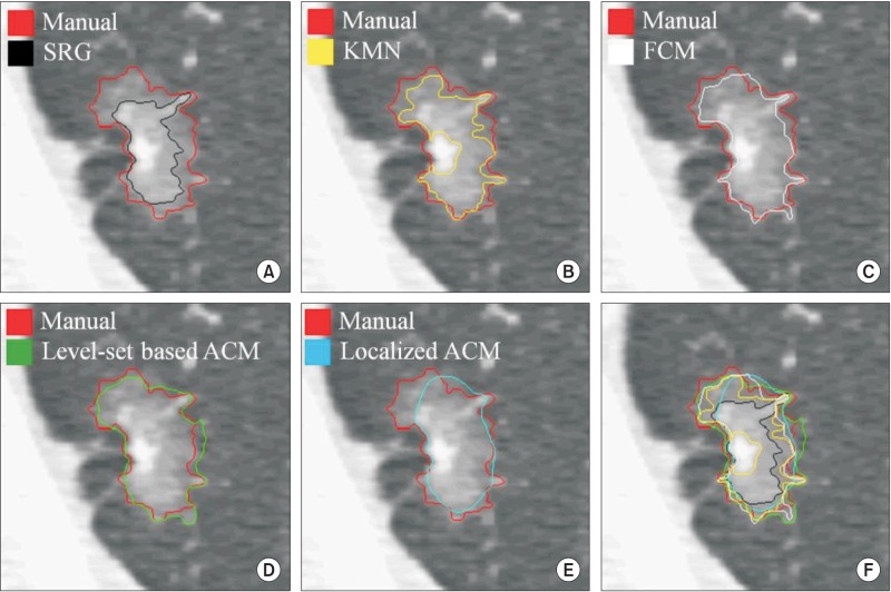
An example of evaluation for segmentation accuracy with the result of manual segmentation (red contour) #1. (A) Seeded region growing (SRG, black), (B) K-means clustering (KMN, yellow), (C) fuzzy C-means clustering (FCM, white), (D) level-set based active contour model (Level-set based ACM, green), (E) localized region-based active contour model (Localized ACM, blue), and (F) overall comparison of accuracy for each method with boundary overlay.

Figure 4

An example of evaluation for segmentation accuracy with the result of manual segmentation (red contour) #2. (A) Seeded region growing (SRG, black), (B) K-means clustering (KMN, yellow), (C) fuzzy C-means clustering (FCM, white), (D) level-set based active contour model (Level-set based ACM, green), (E) localized region-based active contour model (Localized ACM, blue), and (F) overall comparison of accuracy for each method with boundary overlay.

In case of Figures 3F and 4F, they represent overlay images of boundaries regarding the segmented objects with different colors. In these cases, we can confirm that the results of the level-set-based active contour model are most similar to the results of manual segmentation. After binarization, each segmented object was used to calculate the Dice coefficient in the quantitative evaluation step.

2. The Result of Similarity Calculation

To evaluate the accuracy of segmentation with a more objective and quantitative index, we measured image similarity. Table 1 shows the measurement results. In this test, we calculated the Dice coefficient among the results of the manual and semi-automatic segmentation.

Table 1

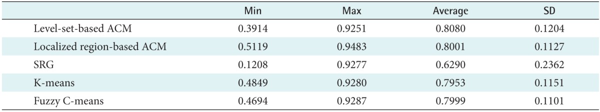
The result of the Dice coefficient calculation from 40 GGNs in CT images

The average Dice coefficient for the methods were 0.8080 for the level-set-based active contour model, 0.8001 for the localized region-based active contour model, 0.6290 for seeded region growing, 0.7953 for K-means clustering, and 0.7999 for the fuzzy C-means clustering, respectively. Consequently, the best result was achieved by the level-set-based active contour model with a maximum Dice coefficient of 0.9251.

Figure 5 presents the result of the ROC analysis for each image segmentation method. We set the level of significance to 95%. The results demonstrate that the level-set-based active contour model achieved the best accuracy.

Figure 5

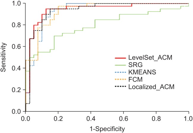
The result of the ROC analysis. Each line is represented in different colors according to the method as follows: the level-set based active contour model (LevelSet_ACM, red), the localized region-based active contour model (Localized_ACM, black dotted), the seeded region growing (SRG, green), the K-means clustering (KMEANS, blue dotted), and the fuzzy C-means clustering (FCM, yellow dotted).

Table 2 shows the result of the AUC analysis, and the best result was also achieved by the level-set-based active contour model with 0.943.

Table 2

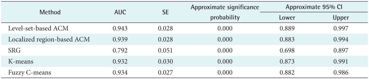
The result of the AUC calculation

Therefore, of the five methods considered, we found that this method achieved the results that were closest to those obtained by manual segmentation for GGN regions. In the case of SRG, on the other hand, we found that it has some discriminant power, but it is difficult to apply to practical trials with the lowest accuracy (AUC = 0.792) values.

IV. Discussion

GGN is a nonspecific finding that may be caused by various disorders. When GGNs are persistent over follow-ups, the probability of lung cancer can be substantially high. Nakata et al. [3] reported that 79.1% of persistent GGNs were lung cancer, which were pathologically proven to be BAC (53.5%), adenocarcinoma with mixed bronchioloalveolar carcinoma components (25.6%), respectively. Moreover, the malignancy rate of GGN lesions was approximately 93% when the lesions contained a solid component.

In a similar study, Kim et al. [28] also assessed 53 GGNs in terms of nodule size, shape, contour, internal characteristics, and the presence of a pleural tag. They compared the findings with histopathological results. In their study, about 75% of persistent GGNs were attributed to BAC or adenocarcinoma with a BAC component.

Despite these potential clinical significances, persistent GGNs are still often missed by CT screenings because the lesions are represented by low attenuation and are faint. The discrimination of malignant nodules from benign tumors is also difficult, although thin-section CT has been widely used. Fortunately, useful computerized image processing techniques have been used in the detection and characterization of persistent GGNs in recent times.

In our study, to extract persistent GGNs, which are often considered an important marker in lung cancer diagnosis through CT images, we attempted to find an effective segmentation method following a detection step. To do this, we performed a comparative study to evaluate segmentation accuracy of five segmentation methods that are widely used for medical image segmentation. Of course, medical images generally show a large degree of variability. For this reason, we selected and applied semi-automatic segmentation methods rather than fully automatic methods.

In the case of seeded region growing, it has its own advantage in that it can be applied easily and fast. However, we expected that it would be difficult to apply to extraction in a microstructure region such as a GGN, because it only considers pixel intensity and shows different results depending on the position of the initial seed point. Moreover, the results of the practical test also showed the lowest suitability.

In the case of two clustering-based methods, they showed more stable results than the SRG method. However, they also demonstrated different results depending on the number of initial clusters or the variability of sample points, so there still remains a limitation.

On the contrary, the level-set-based active contour model has advantages whereby it is possible to segment a very small ROI region, such as a GGN at high speed, and multiply when various objects exist in an image. It is expected to obtain results.

The localized region-based active contour model is known to provide robustness against initial curve position and insensitivity to image noise. With such advantages, this method has been used to segment thyroid nodules in ultrasound and scintigraphy images recently. Therefore, we expected to get better results when we selected and applied it to GGN images. However, our test showed that it achieved rather lower segmentation performance compared to the level-set-based active contour method.

In the present study, we did not include the segmentation of multiple objects in an image because we only focused on segmentation accuracy. That being said, we will surely consider that aspect in our future studies. Although it demonstrated great potential as to its application in helping specialists extract the correct GGN region, our methodology still requires the use of other techniques.

Firstly, some ROI images were magnified with proper sizes for our test because their original object sizes were very small. Some of them showed data losses regarding intensity information including object boundaries, to a greater or lesser extent. For this reason, these data showed the results of under- or over-segmentation as shown in Figure 6. For example, Figure 6A shows the result of the segmentation by the level-set-based active contour method (practically this data was not included our test).

Figure 6

An example of over-segmentation and under-segmentation: (A) under segmented region in the segmentation with the level-set based active contour model (yellow regions); (B) over segmented region in the segmentation with the seeded region growing (red regions).

Although we obtained a mean Dice coefficient of 0.8080, it also represents the same issue at parts of an image. Therefore, we believe that a more improved method is required, which can preserve edges effectively on the segmentation of microstructure regions. It is expected that we can greatly improve the overall accuracy of segmentation if we use more adaptive methods.

The number of patients’ images did not allow us to carry out more precise analyses to ascertain the total efficiency of the methods. Thus, it is necessary to deepen our present analysis with a larger and more balanced image base of patients. Also, it is important to use other images, obtained under different acquisition protocols to better evaluate the behavior of the present methods. In addition, we did not attempt to segment GGNs, which were represented by multiple nodules on thin-section CT scans. However, we expect to achieve it easily after appropriate parameter settings because one characteristic of the level-set-based active contour model is that it allows us to extract multiple objects simultaneously.

In conclusion, we hope to extend the present methods to the study of GGN detection and segmentation in 3D space. To analyze objects, which have 3D characteristics in nature, we believe that 3D-based methods, which could minimize the loss of information compared with 2D-based methods, are more suitable. Furthermore, we also believe that it is more effective in terms of time and cost. As reported in many recent studies, research on 3D CAD systems and various related technologies continues to be as vigorous as ever [29 30].

Although various image segmentation methods have been developed in many studies, they have considered the 'trade-off' between speed and accuracy as an important common problem. We think our study should help to establish a proper standard for accuracy and speed for segmentation. Thoughtful consideration of this problem is very important for clinical diagnosis.

Acknowledgments

This work was supported by a research grant from the National Cancer Center, Korea (Grant No. 1610050-1).

Notes

Conflict of Interest: No potential conflict of interest relevant to this article was reported.

References

1. Siegel R, Ward E, Brawley O, Jemal A. Cancer statistics, 2011: the impact of eliminating socioeconomic and racial disparities on premature cancer deaths. CA Cancer J Clin 2011;61(4):212–236. 21685461.

2. Song JS, Kim SY, Jo HJ, Lee KK, Shin JH, Shin SN, et al. The role and significance of biomarker for plasma G-CSF in patients with primary lung cancer. Tuberc Respir Dis 2009;66(6):444–450.

3. Nakata M, Saeki H, Takata I, Segawa Y, Mogami H, Mandai K, et al. Focal ground-glass opacity detected by low-dose helical CT. Chest 2002;121(5):1464–1467. 12006429.

4. Beasley MB, Brambilla E, Travis WD. The 2004 World Health Organization classification of lung tumors. Semin Roentgenol 2005;40(2):90–97. 15898407.

5. Park CM, Goo JM, Lee HJ, Lee CH, Chun EJ, Im JG. Nodular ground-glass opacity at thin-section CT: histologic correlation and evaluation of change at follow-up. Radiographics 2007;27(2):391–408. 17374860.

6. Lee HY, Lee KS. Ground-glass opacity nodules: histopathology, imaging evaluation, and clinical implications. J Thorac Imaging 2011;26(2):106–118. 21508733.

7. Godoy MC, Naidich DP. Subsolid pulmonary nodules and the spectrum of peripheral adenocarcinomas of the lung: recommended interim guidelines for assessment and management. Radiology 2009;253(3):606–622. 19952025.

8. Bastawrous HA, Nitta N, Tsudagawa M. A new CAD system for detecting localized ground glass opacity nodules in lung CT images using cross and coronary section images In : Proceedings of IEEE International Workshop on Medical Measurement and Applications; 2006 Apr 20-21; Benevento, Italy. p. 54–57.

9. Kim KG, Goo JM, Kim JH, Lee HJ, Min BG, Bae KT, et al. Computer-aided diagnosis of localized ground-glass opacity in the lung at CT: initial experience. Radiology 2005;237(2):657–661. 16192320.

10. Li Q, Li F, Doi K. Computerized detection of lung nodules in thin-section CT images by use of selective enhancement filters and an automated rule-based classifier. Acad Radiol 2008;15(2):165–175. 18206615.

11. Kanazawa K, Kubo M, Niki N, Satoh H, Ohmatsu H, Eguchi K, et al. Computer assisted lung cancer diagnosis based on helical images In : Proceedings of 3rd International Computer Science Conference; 1995 Dec 11-13; Hong Kong. p. 323–330.

12. Okumura T, Miwa T, Kako JI, Yamamoto S, Matsumoto M, Tateno Y, et al. Image processing for computer-aided diagnosis of lung cancer screening system by CT (LSCT). Proc SPIE Int Soc Opt Eng 1998;3338:1314–1322.

13. Zhou J, Chang S, Metaxas DN, Zhao B, Ginsberg MS, Schwartz LH. An automatic method for ground glass opacity nodule detection and segmentation from CT studies. Conf Proc IEEE Eng Med Biol Soc 2006;1:3062–3065. 17946543.

14. Kim H, Katsumata Y, Tan JK, Ishikawa S. Automatic detection of GGO in CT lung images by using statistical features and neural networks In : Proceedings of International Technical Conference on Circuits Systems, Computers and Communication (ITC-CSCC); 2009 Jul 5-8; Jeju, Korea. p. 705–708.

15. Bastawrous HA, Fukumoto T, Nitta N, Tsudagawa M. Detection of ground glass opacities in lung CT images using Gabor filters and neural networks In : Proceedings of IEEE Instrumentation and Measurement Technology Conference; 2005 May 16-19; Ottawa, Canada. p. 251–256.

16. Ikeda K, Awai K, Mori T, Kawanaka K, Yamashita Y, Nomori H. Differential diagnosis of ground-glass opacity nodules: CT number analysis by three-dimensional computerized quantification. Chest 2007;132(3):984–990. 17573486.

17. Tomasi C, Manduchi R. Bilateral filtering for gray and color images In : Proceedings of 6th International Conference on Computer Vision; 1998 Jan 4-7; Bombay, India. p. 839–846.

18. Barash D. Bilateral filtering and anisotropic diffusion: towards a unified viewpoint In : Proceedings of 3rd International Conference on Scale-Space; 2001 Jul 7-8; Vancouver, Canada. p. 273–280.

19. Caselles V, Catte F, Coll T, Dibos F. A geometric model for active contours in image processing. Numer Math 1993;66(1):1–31.

20. Sethian JA. A fast marching level set method for monotonically advancing fronts. Proc Natl Acad Sci U S A 1996;93(4):1591–1595. 11607632.

21. Shyu KK, Pham VT, Tran TT, Lee PL. Global and local fuzzy energy-based active contours for image segmentation. Nonlinear Dyn 2012;67(2):1559–1578.

22. Li C, Xu C, Gui C, Fox MD. Level set evolution without re-initialization: a new variational formulation In : Proceedings of 2005 IEEE Computer Society Conference on Computer Vision and Pattern Recognition; 2005 Jun 20-25; San Diego, CA. p. 430–436.

23. Lankton S, Tannenbaum A. Localizing region-based active contours. IEEE Trans Image Process 2008;17(11):2029–2039. 18854247.

24. Kaur J, Jindal A. Comparison of thyroid segmentation algorithms in ultrasound and scintigraphy images. Int J Comput Appl 2012;50(23):24–27.

25. Mingoti SA, Lima JO. Comparing SOM neural network with fuzzy C-means, k-means and traditional hierarchical clustering algorithms. Eur J Oper Res 2006;174(3):1742–1759.

26. Zijdenbos AP, Dawant BM, Margolin RA, Palmer AC. Morphometric analysis of white matter lesions in MR images: method and validation. IEEE Trans Med Imaging 1994;13(4):716–724. 18218550.

27. Fawcett T. An introduction to ROC analysis. Pattern Recognit Lett 2006;27(8):861–874.

28. Kim HY, Shim YM, Lee KS, Han J, Yi CA, Kim YK. Persistent pulmonary nodular ground-glass opacity at thin-section CT: histopathologic comparisons. Radiology 2007;245(1):267–275. 17885195.

29. Tang L, Kwon YH, Alward WL, Greenlee EC, Lee K, Garvin MK, et al. 3D reconstruction of the optic nerve head using stereo fundus images for computer-aided diagnosis of glaucoma. Proc SPIE Int Soc Opt Eng 2010;7624:76243.

30. Way TW, Hadjiiski LM, Sahiner B, Chan HP, Cascade PN, Kazerooni EA, et al. Computer-aided diagnosis of pulmonary nodules on CT scans: segmentation and classification using 3D active contours. Med Phys 2006;33(7):2323–2337. 16898434.

Article information Continued

(open-access, http://creativecommons.org/licenses/by-nc/4.0/) :

This is an Open Access article distributed under the terms of the Creative Commons Attribution Non-Commercial License (http://creativecommons.org/licenses/by-nc/4.0/) which permits unrestricted non-commercial use, distribution, and reproduction in any medium, provided the original work is properly cited.

Funded by : National Cancer Centerhttp://dx.doi.org/10.13039/501100003645

Award ID : 1610050-1