Real-Time Computed Tomography Volume Visualization with Ambient Occlusion of Hand-Drawn Transfer Function Using Local Vicinity Statistic
Article information
Abstract
Objectives
In this paper, we present an efficient method to visualize computed tomography (CT) datasets using ambient occlusion, which is a global illumination technique that adds depth cues to the output image. We can change the transfer function (TF) for volume rendering and generate output images in real time.
Methods
In preprocessing, the mean and standard deviation of each local vicinity are calculated. During rendering, the ambient light intensity is calculated. The calculation is accelerated on the assumption that the CT value of the local vicinity of each point follows the normal distribution. We approximate complex TF forms with a smaller number of connected line segments to achieve additional acceleration. Ambient occlusion is combined with the existing local illumination technique to produce images with depth in real time.
Results
We tested the proposed method on various CT datasets using hand-drawn TFs. The proposed method enabled real-time rendering that was approximately 40 times faster than the previous method. As a result of comparing the output image quality with that of the conventional method, the average signal-to-noise ratio was approximately 40 dB, and the image quality did not significantly deteriorate.
Conclusions
When rendering CT images with various TFs, the proposed method generated depth-sensing images in real time.
I. Introduction
Computed tomography (CT) is an imaging procedure that uses X-ray technology to produce tomographic images of a specific object. Volume visualization [12] is a technique to visualize three-dimensional arrays of voxels, including CT datasets.
Ray casting [134], which is a general method of volume visualization, virtually fires a ray from each pixel of an output image and calculates the color of the ray passing through the volume data (Figure 1). The CT value (or voxel value) is the X-ray absorbance of the human organ tissue. The CT value of a sample is transformed into color and opacity through a user-defined transfer function (TF) [5]. The sample color is then changed more realistically according to lighting effects [6], and the final color for a ray is determined as the result of accumulation of samples.
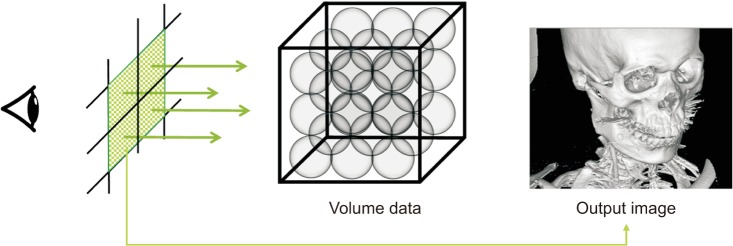
Ray casting method. The rays originating from each pixel pass through the volume data. The accumulated pixel color is output as the final image.
To generate high-quality images, there are many research areas corresponding to each stage of the volume rendering pipeline, such as sampling [7], TF design [8], and illumination [9]. Traditional local illumination [6] reveals the shape of objects, but it lacks depth cues and is sensitive to local noise; therefore, global illumination can be considered as a complementary method.
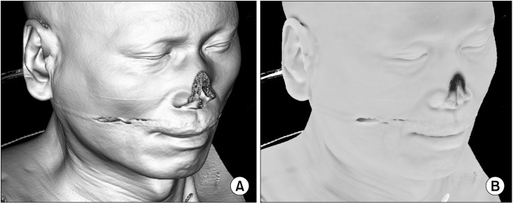
Global illumination is a powerful lighting effect used to generate more realistic lighting. Ambient occlusion [10111213] is a global illumination technique that detects and darkens indentations on an object, such as wrinkles or holes (Figure 2). By adding ambient occlusion to traditional volume visualization, we can improve depth cues. Because of the large computational overhead, ambient occlusion requires hours of pre-computation [10] or is applied applied in fixed TF environments [11]. Another method performs ambient occlusion at high speed by performing depth estimation in an image space [12], but it is difficult to apply to translucent data. In our previous research [14], the above problem was partially solved, and the TF could be changed in real time. However, the derivation of the equation for ambient occlusion was assumed when the TF is trapezoidal in [14]. In this study, we derived a new equation for a general piecewise linear TF to use the ambient occlusion technique for the volume dataset. Moreover, we applied additional methods to reduce the number of line segments because the computation time of the new equation is proportional to the number. Thus, real-time ambient occlusion is performed using the general forms of TFs, such as hand-drawn curves.
II. Methods
The local vicinity of each voxel is generated in the preprocessing step and ambient occlusion is performed using a hand-drawn TF in the visualization step. Additionally, we simplify the TF to enable high-speed visualization.
In the preprocessing step, we calculate the mean and standard deviation of the local vicinity by applying our previous method [14] without modification; it is introduced in Section II-1. The ambient occlusion that we propose is calculated in the rendering step described in Section II-2. The technique for smoothing and simplifying the TF is described in Section II-3. The overall algorithm is shown in Figure 3.
1. Fast Calculation of Local Vicinity Information
In this study, we assumed that the CT value near an arbitrary point follows the normal distribution. The average and standard deviation of the values of the n × n × n-sized region around each voxel should first be obtained. In general, the computational complexity for each voxel is O(n3), but it can be calculated in O(1). The incremental algorithm for the average value of each region is calculated as follows [14]:
(i) The sum of the CT values of the n × 1 × 1 region around the voxel position (s, t, u) is calculated and stored as Sum1D(s, t, u).
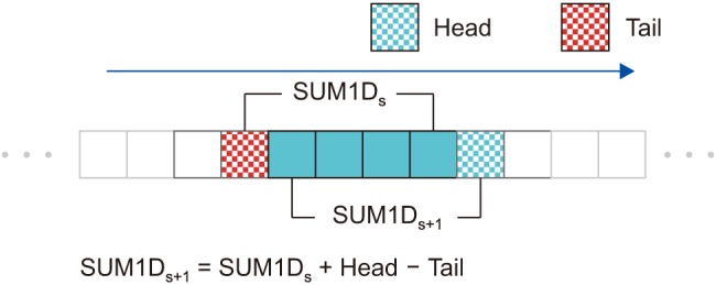
(ii) The region for the next position, (s + 1, t, u), is overlapped with the previous region by (n − 1) × 1 ×1 (Figure 4). Therefore, the next sum can be calculated in O(1) as
Sum1D(s, t + 1, u) = Sum1D(s, t, u) + Head1D − Tail1D

(iii) Sum2D(s, t, u), which is the sum of the n × n × 1 region, can be obtained by adding the Sum1D values. As Sum2D(s, t, + 1, u) is overlapped with Sum2D(s, t, u) by n × (n − 1) × 1, the calculation is also in O(1) as
Sum2D(s+1, t, u) = Sum2D(s, t, u) + Head2D − Tail2D

(iv) Sum3D(s, t, u + 1) is calculated in O(1) in the same way. Finally, the average value of the n × n × n region is Avg3D(s, t, u) := Sum3D(s, t, u)/n3.
By squaring each CT value, creating a new volume, and repeating the above procedure, we obtain SquaredAvg3D(s, t, u), which is the average of the squared values. The variance, which is the square of the standard deviation, is generated using the following equation:
In this way, the average and standard deviation of the n × n × n region centered on one voxel are calculated in constant time.
2. High-Speed Ambient Occlusion Volume Rendering Algorithm
The ambient occlusion method measures how much the surrounding objects occlude and shade a sample at each position. If the surroundings are transparent, the sample becomes bright because the light is not obscured; if opaque, the sample becomes dark:

For a sample position, the ambient occlusion value is the sum of each opacity multiplied both by the opacity a(x) of the CT value x and by the probability ρ(x) that x exists in the vicinity of the sample. Equation (4) is simplified to be independent of the distance between the sample position and the local vicinity [14].
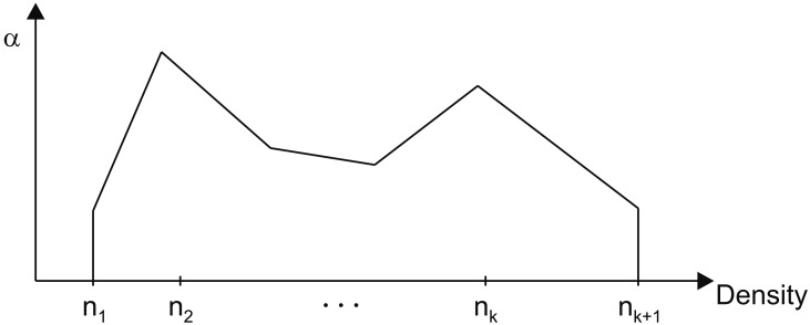
In previous research, the TF was usually a rectangular shape [1414], but it can be piecewise linear [1516], curved [17], or drawn by hand [18]. The generalized one-dimensional TF shown in Figure 5 can be expressed with a connection of k line segments as

In this study, we assumed that the CT value around each voxel follows the normal distribution, N(m, σ2). If ρ(x) is N(0, 1), we are able to derive Equations (6) and (7) from Equations (4) and (5) as

where

In Equation (7), N(x) is a cumulative standard normal distribution obtained by integrating the standard normal distribution. As we calculated and stored the value of N(x) for each x as a lookup table, the number of calculations for Equation (6) is O(k).
If ρ(x) is the normal distribution N(m, σ2), the ambient occlusion is calculated using a normalized variable transformation  or x = σz + m. Each line segment of the TF is then transformed as follows:
ai(x) = aix + bi = ai(σz + m) + bi = (σai)z + (bi + aim)

For example, if we assume that there is a user-drawn TF like that in Figure 5 and the first line segment passes through two control points, (110, 0.1) and (130, 0.3), then the equation of the line is a1(x) = 0.01x − 1. If the mean and variance of the n × n × n region centered on a sample are m = 120 and σ2 = 102, respectively, the ambient occlusion of the first TF segment is calculated as

If the second line segment passes through (130, 0.3) and (150, 0.7), then a2(x) = 0.02x − 2.3:

The sum of all Segi values is the ambient occlusion value for a sample. The closer the sum is to 1.0, the darker the sample is. Using the basic method in Equation (4), 4096 iterations are needed for 12-bit CT precision. In comparison, the proposed method requires only k (the number of TF line segments) iterations, thereby greatly reducing the total computational overhead.
3. TF Simplification
The computational cost of the proposed equation is proportional to the number of line segments in the TF. Because the hand-drawn TF has many vertices and connecting lines, we simplified it to a small number of line segments to improve performance. For this, we used the method of Hadwiger et al. [19], by which an error tolerance (a window) is defined for every vertex. Simplified line segments must pass through the windows of the input vertices, as shown in Figure 6. The algorithm is calculated as follows:

Transfer function (TF) simplification method: (A) inputting TF, (B) finding the longest line starting at p0 through as many consecutive windows as possible, and (C) creating the next starting point and repeating the process.
1) Connect the starting point (s) to the window (red line) of the next point to obtain the slope range (green line).
2) Move the target to the next point and reduce the slope range so the line segment passes through the new window (w2, w3).
3) If we cannot pass the next window (p4) in the current range, a new starting point is created, and we return to step 1.
If the user draws the TF by hand using a touch screen or mouse, hand tremors may produce unintentionally sharp graphs, which deteriorate the output image, increase the number of line segments, and reduce the rendering speed. In this study, noise was removed by pre-filtering when a hand-drawn TF was used. Through experiments, we found that an average filter with a kernel size of 5 was suitable.
III. Results
The development and experiment of this study was performed on a PC equipped with an Intel Q9550 CPU, 4 GB RAM, and GeForce GTX 1050 GPU. We used four CT datasets (HEAD, ABDOMEN, LOWER, and LIVER) as shown in Table 1. The region size (n × n × n) was 15 × 15 × 15. We implemented ray casting using GPU programming [20] and applied accelerating techniques, empty space skipping, and early ray termination [4].
In Figure 7, image column (A) shows the results of existing local illumination [3], while column (B) shows results of the proposed ambient occlusion method described in Section 2.2. Image column (C) depicts a mixing of the images in (A) and (B), and column (D) is the result of additional acceleration, as described in Section II-3.
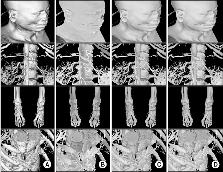
Results of various rendering methods for volume datasets (HEAD, ABDOMEN, LOWER, and LIVER): (A) previous local illumination, (B) proposed ambient occlusion (Section II-2), (C) weighted average of (A) and (B), and (D) accelerated method (Section II-3) of (C).
Also, in Figure 7, image column (A) shows the surface texture clearly, while column (B) reveals the sense of space and depth. The ambient occlusion technique complements existing local illumination techniques. For example, the depth of the human ear is distorted in HEAD (A) and more sensibly depicted in HEAD (B). The spaces between vertebrae are smoother in ABDOMEN (B) than in ABDOMEN (A). The joint surfaces in LOWER (B) are less noisy than those in LOWER (A). Similarly, the liver surfaces in LIVER (B) are less noisy than those in LIVER (A). The advantages of local and global illumination are combined in column (C). Using the acceleration method, high-quality images (Figure 7D) can be produced in real time.
Next, we evaluated the performance of the proposed method. As the proposed method is a natural extension of the existing method [14], they generated the same image when the TF was trapezoidal. Additionally, our method was able to handle hand-drawn TFs. Image column (D) is the combined result of the two acceleration methods. Using Equation (3) presented in Section II-2, the 4096 iterations for a 12-bit CT dataset were reduced to hundreds without degradation of image quality. If a slight difference in the lighting effect is allowed, the number of iterations can be reduced to dozens using the simplification method presented in Section II-3.
The upper line in Figure 8A is a TF used to visualize HEAD data, and it consists of a number of line segments—similar to the TF in Figure 5. As described in Section II-3, increasing the window size reduces the number of approximate segments, such that the rendering speed increases and image quality degrades. As shown in Figure 8B, as the window size increased, the number of line segments of the simplified TF (blue line) and the image quality decreased (red line).

(A) Hand drawn TF and (B) comparison of image quality for the proposed method. Upper line is for the HEAD dataset, and lower line is for the ABDOMEN, LOWER, and LIVER datasets. As the window size increases, the line segment quantity, which translates into computational time, and image quality (SNR) decrease. When the window size is approximately 10, we obtain relatively high-quality images (high SNR) in a short time. CT: computed tomography, TF: transfer function, SNR: signal-to-noise ratio.
The bottom graph in Figure 8A shows a TF used to visualize ABDOMEN, LOWER, and LIVER data. The bottom graph in Figure 8B shows the changes in the image quality and number of line segments according to the change in window size. As the window size increased, the number of line segments sharply decreased and gradually stabilized at a window size of 10. Image quality tended to decrease as the window size increased for each dataset.
Table 2 shows the rendering time and signal-to-noise ratio (SNR) values after a window size of 8 was applied. Using the simplification method proposed in this study, the visualization performance was improved by approximately 40 times. The resulting image had an SNR value of approximately 40 dB and was difficult to differentiate from the original.
IV. Discussion
In this paper, we proposed an efficient ambient occlusion method for CT volume visualization. Our results showed better spatial and depth cues in the output images because the rendering method considers the transparency around each sample.
In previous research, a significant amount of time was required to calculate the transparency of the local vicinity for each sample; therefore, real-time rendering was not possible except for static scenes with fixed TFs. In our previous research, the TF was changeable only when trapezoidal.
We can now handle a TF composed of an arbitrary number of line segments. We have derived a method to reduce the number of calculations from the CT value range (4096, 12-bit) to the number of line segments (a few hundred or less) without affecting the result. In the next step, we further improved the performance without explicit quality differences using approximation methods that reduce the number of line segments. The proposed two-step acceleration method improves performance by 40 times and enables real-time rendering using ambient occlusion.
The proposed TF simplification method produces a visually comparable image. This method can reduce the noise in TF graphs caused by human hand tremors. As the ambient occlusion technique generates low-frequency images and only affects the lighting, the proposed simplification method does not impact diagnosis and image quality.
A limitation of our research is that the CT value around a sample was assumed to follow the normal distribution. If the distribution of actual data differs greatly from normal distribution (such as in a binary image), a difference in the lighting effect occurs in the output image. For example, there are two regions of CT values, namely, (20, 20, 70, 20, and 20) and (0, 20, 30, 40, and 60). Assuming that the voxel is transparent when its value is less than 25, four voxels in the first region and two voxels in the second are transparent. The first region should be brighter than second because more samples are transparent and do not occlude ambient light. However, as the mean and standard deviation of the two regions are the same (mean = 30, standard deviation = 20), our method generates the same ambient light for each region. For more accurate lighting effects, it would be necessary to consider various data distributions beyond the normal distribution in future work.
Acknowledgments
This work was supported by the National Research Foundation of Korea (NRF) grant funded by the Korea government (Ministry of Science and ICT) (No. 2017R1E1A1A03070494) (Jaewoo Kim). This research was financially supported by Hansung University (Heewon Kye).
Notes
Conflict of Interest: No potential conflict of interest relevant to this article was reported.

